AEI Market Trends Report Sources and Methodologies
Last Updated: 6/4/2020
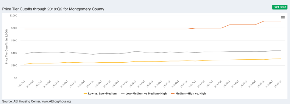
Graphic 1. Price Tier Cutoffs
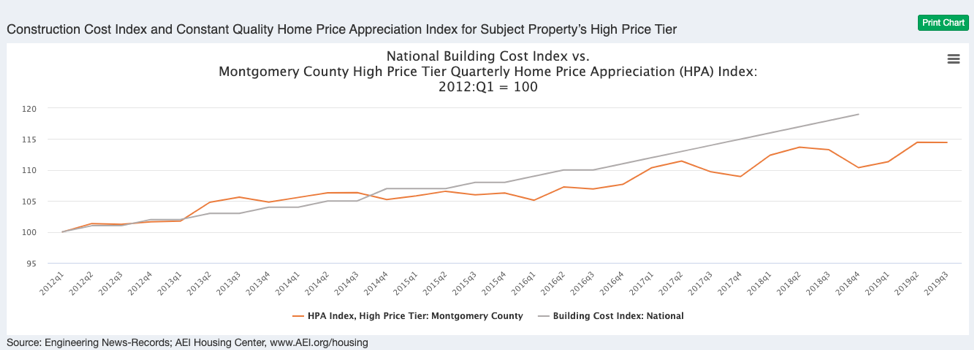
Graphic 2. Construction Cost Index and Constant Quality Home Price Appreciation Index
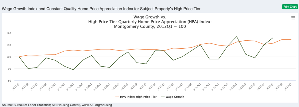
Graphic 3: Wage Growth Index and Constant Quality Home Price Appreciation Index
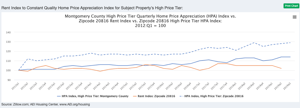
Graphic 4:Rent Index to Constant Quality Home Price Appreciation Index
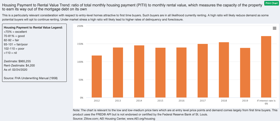
Graphic 5: Housing Payment to Rental Value Trend Housing Payment to Rental Value
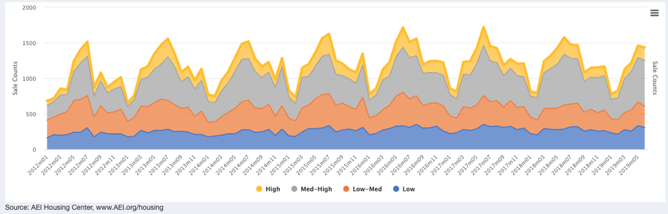
Graphic 6: Public Record Monthly Home Sale Counts by Price Tier
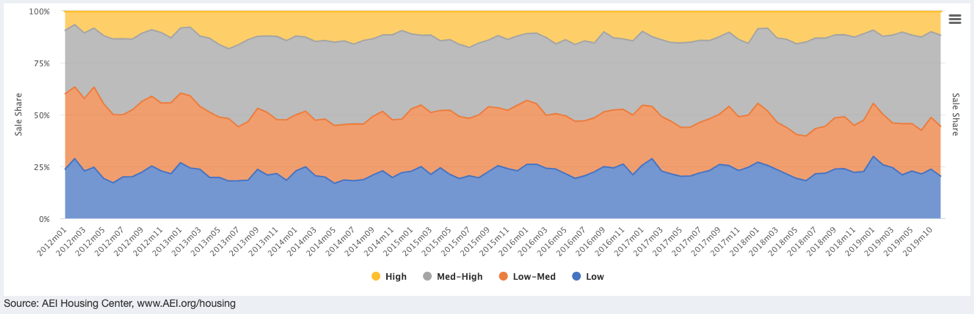
Graphic 7: Public Record Monthly Home Sale Share by Price Tier
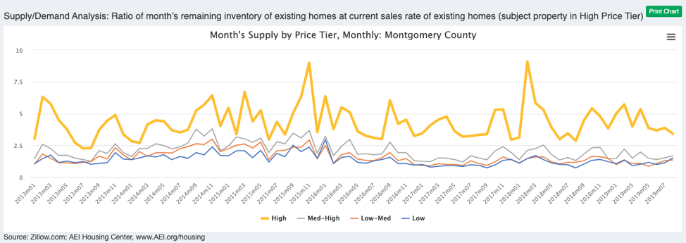
Graphic 8: Supply/Demand Analysis
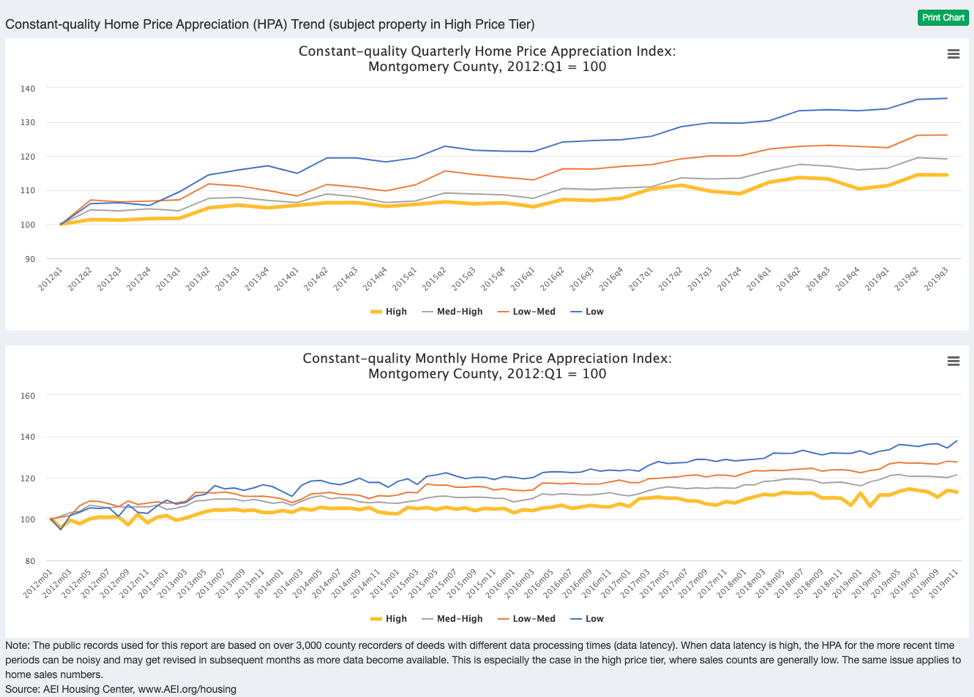
Graphic 9: Quarterly and Monthly Constant Quality Home Price Appreciation (HPA) Trend by Price Tier
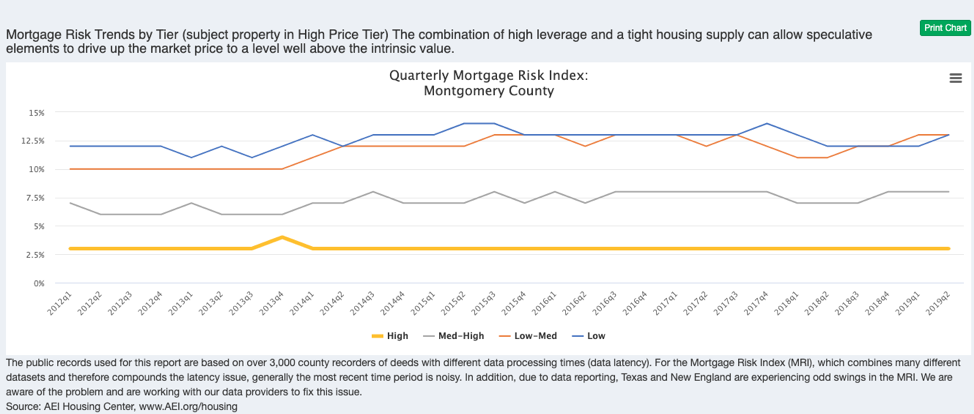
Graphic 10: Mortgage Risk Trends by Price Tier
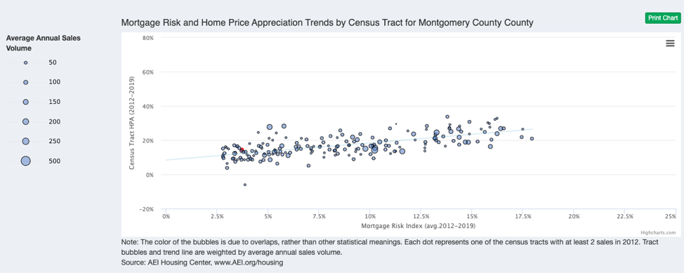
Graphic 11: Mortgage Risk and Home Price Appreciation Trends by Census Tract
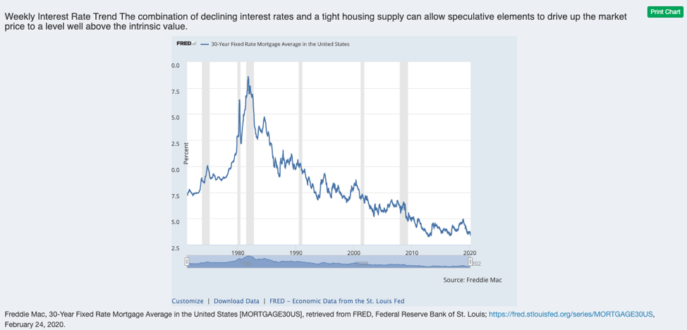
Graphic 12: Weekly Interest Rate Trend
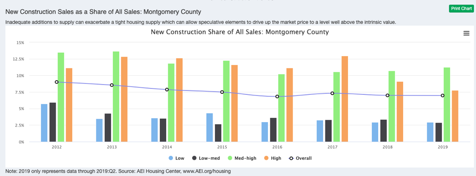
Graphic 13: New Construction Sales as a Share of All Sales
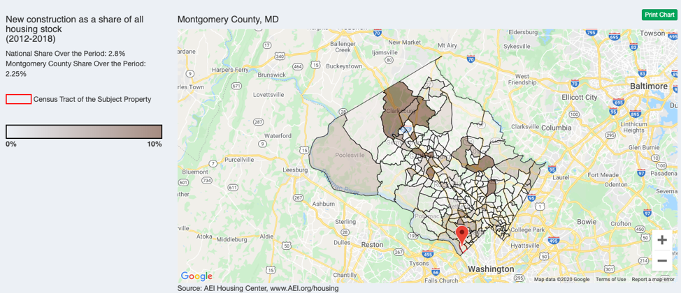
Graphic 14: New construction as a Share of All Housing Stock
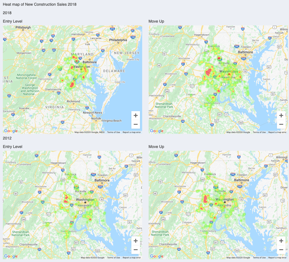
Graphic 15: Heat Map of New Construction Sales
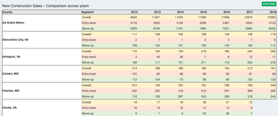
Graphic 16: New Construction Sales -Comparison across Years (Table demonstrates a portion of DC metro)
Section 1: County Merge of Virginia Enclaves
We account for low sales counts in Virginia independent cities and some smaller counties by combining these entities with their surrounding counties. The housing market indicators in these entities are the combined average of the smaller and the larger absorbing county. The table below shows all the changes:
Independent city or small county: |
Absorbing county: |
Bristol, VA |
Washington, VA |
Buena Vista, VA |
Rockbridge, VA |
Charlottesville, VA |
Albemarle, VA |
Colonial Heights, VA |
Chesterfield, VA |
Covington, VA |
Alleghany, VA |
Emporia, VA |
Greensville, VA |
Fairfax City, VA |
Fairfax, VA |
Falls Church, VA |
Fairfax, VA |
Franklin, VA |
Isle of Wight, VA |
Fredericksburg, VA |
Spotsylvania, VA |
Galax, VA |
Carroll, VA |
Harrisonburg, VA |
Rockingham, VA |
Hopewell, VA |
Prince George, VA |
Lexington, VA |
Rockbridge, VA |
Manassas, VA |
Prince William, VA |
Manassas Park, VA |
Prince William, VA |
Martinsville, VA |
Henry, VA |
Norton, VA |
Wise, VA |
Radford, VA |
Montgomery, VA |
Roanoke City, VA |
Roanoke, VA |
Salem, VA |
Roanoke, VA |
Staunton, VA |
Augusta, VA |
Waynesboro, VA |
Augusta, VA |
Winchester, VA |
Frederick, VA |
Section 2: Price Tier Data and Methodology
The four tiers are set at the metro level (see Section 11)1, adjusted quarterly, and defined as follows:
The price tiers are set at these levels to both reflect access to leverage and provide an approximate price point between entry-level homes (Low and Low-Medium) and move-up homes (Medium-High and High).
Price tiers are based on sale price not the loan limits themselves because houses are sold based on price and not loan amount.
The main data source to compute the 40th and 80th percentile of FHA sale price is the FHA Snapshot data, which is a census of FHA loan endorsements.2 The key variables used from these data are loan amount, county code, and endorsement month. We account for the difference between origination/sale date and endorsement date (in the Snapshot data), by assuming that the FHA endorses the loan one month after its origination.
To convert loan amount to sale price we assume a CLTV of 98.2% (96.5% plus 1.75% upfront mortgage insurance premium (MIP)).
The GSE loan limits come from FHFA and take into account for high-cost area limits. To convert loan amount to sale price we assume an LTV of 80%, which, according to NMRI data, is the most commonly used LTV by GSE borrowers at the applicable loan limit. At such an LTV, we divide the CLL by .8 or multiply the CLL by 1.25 to arrive at the sale price cutoff.
The price tiers represent roughly the following percentages of national financed home sales:
(Percentages shown are averages for 2018.)
The FHA Snapshot data are released with a lag of 1-2 months, which increases by another month to account for the endorsement date lag. Graphic 1, however, will show data through the most recent quarter. Thus, the FHA price percentiles for the most and perhaps the second to last quarter are estimated based on prior year’s trends.
Every sale is assigned a price tier. For sales for which a sale price is missing (~7% of the total), we default to the Automated Valuation Model (AVM) value to assign a price tier.3 If that is unavailable as well, we query the Zillow Zestimate and adjust it using our HPA index for a possible sale price at purchase. The potential for error is small as the price tier ranges are large. For only a small number of sales (<0.1%) a price tier is unavailable.
Section 3: Constant Quality Home Price Appreciation (HPA) Methodology
Basics of HPA index construction:
HPA is a “quasi” repeat sales index. The index measures HPA by constructing a sales pair consisting of one actual sale and one “quasi sale as measured by the property’s Automated Valuation Model (AVM.) The AVM approximates a property’s sale price at a given point in time. The AVM used has been evaluated by us and has been found to be, on average unbiased and accurate (that is it has a normal error distribution).
Advantages of AEI’s HPA Index:
A true repeat sales index is limited by the number of repeat sale pairs, which limits the ability to determine HPA trends at finer geographies. AEI’s index includes the entire universe of sales. Since this approach has many more data points, it allows for index construction by price tier across many more metros and at fine geographic levels (down to census tract). Finally, a true repeat sales index may introduce a bias towards properties that sell more frequently, thereby allowing them to constitute a greater portion of the repeat sales pairs.
Data for the HPA index:
National Public Records data and AVM for Dec-2018 come from First American via DataTree.com. The index uses virtually all institutionally financed sales back to January 2012. Data are weighted at the county level to adjust for minor amounts of missing data. HPAs for the medium-high and high price tiers are spliced around the time of loan limit changes. Data exclude new construction sales, sales of distressed properties, and sales of properties that sold multiple times within a one-year period. The current dataset includes 16 million purchase transactions as of January 2019 and will expand as new sales are accumulated going forward. HPA data for the most recent month are preliminary.
Section 4: Housing Payment to Rental Value Methodology
This ratio is calculated using total monthly housing payment over rental value, which measures the capacity of the property to earn its way out of the mortgage debt on its own.
Total monthly housing payment includes mortgage principal and interest payment (PI), mortgage insurance premium (MIP), property tax and insurance (TI).
Data for the calculation are:
Zestimate and Rent-Estimate are provided by Zillow.com. They are recent with a lag of 0-2 days.
The other parameters in the housing payment calculation are stylized:
While the above parameters are given in the “current year scenario”, property value, rental value, and mortgage interest rate vary in the following scenarios:
Prior years:
Sale price is retroactively estimated at its value for the 4th quarter of each year. The most recent Zestimate is rolled back in time using AEI’s quarterly home price appreciation series at the county level.
Similarly, the rental value is estimated for the 4th quarter of each year by rolling it in time using the monthly Zillow ZRI Time Series (Multifamily, SFR, Condo/Co-op) at the zip code level.
First payment mortgage rates for prior years are assumed to average weekly rates of the 4th quarter of each year.
"If interest rate is 6%" scenario:
Same as current year but assumes an interest rate of 6%.
This scenario assumes that mortgages rates return to a level closer to, but still well below their long-term average. This scenario is illustrative, but provides guidance on the impact a return to a more normal rate environment. It is especially relevant for entry-level homes (the low- and low-medium price tiers). About 75% of the demand for these tiers comes from first-time buyers and these buyers are largely renters. Thus a substantial increase in the ratio between monthly housing payment and monthly rental value would likely reduce demand for starter homes, while at the same time increasing supply. This would cause the month’s remaining inventory to rise. A large enough rise would likely lead to a decline in home prices.
FHA in the mid-20th century endeavored to quantify this relationship as follows:
Housing Payment to Rental Value Legend:
<70% = excellent
70-81% = good
82-92 = fair
93-101 = fair/poor
102-110 = poor
>110 = nil (FHA set as an automatic turndown)
These values are based on the FHA Underwriting Manual (1958).
Section 5: Home Sales Methodology
Public record monthly home sale counts come from public records data at the county level from First American via Data Tree. There are 2,900 counties and county-equivalents that report such data. In our counts we limit the data to purchase transactions that involve an individual as either a buyer or seller. AEI doesn’t further adjust or weight the numbers using other data sources.
Data are from 2012 to the most recent completed month, and overall cover an estimated 90 percent of the home purchase market. While virtually all counties and county-equivalents are accounted for in the public records data, certain such entities:
For more on the public record data, see Section 10.
Section 6: Months’ Supply Methodology
Months’ supply measures how many months it would take for the inventory of existing homes for sale to be exhausted at the current sales pace. Across all price points, six months is generally considered the demarcation point between a buyer’s and seller’s market.
Inventory is measured by taking daily snapshots of available listings over various points of a month. These data exclude pending home sales. Inventory and existing home sales numbers are aggregated monthly for each AEI price tier (described in Section 2). The data date back to January 2013 and are provided by way of custom runs by Zillow and are not publicly available. Data are provided for over 2,200 counties.
Section 7: Mortgage Risk Index (MRI) Methodology
The matched data (described in Section 1) are risk rated based on the following methodology for the AEI National Mortgage Risk Index (NMRI):
We define a high risk loans as having an MRI of at least 12%, twice the stressed default rate of a low risk loan.
Matched loans, for which a DTI is missing, are assigned the median DTI for that census tract or county, if tract is unavailable. Matched loans with a missing credit score or CLTV are not risk rated.
Overview of methodology
The NMRI measures how the loans originated in a given month would perform if subjected to the same stress as in the financial crisis that began in 2007. This is similar to stress tests routinely performed to ascertain an automobile’s crashworthiness or a building’s ability to withstand severe hurricane force winds. We calculate this stressed mortgage default rate in a series of steps. The details presented immediately below pertain to home purchase loans.
The first step is to create a matrix of benchmark default rates for home purchase loans acquired by Freddie Mac in 2007.10 The Freddie Mac data used for this calculation consist of 30-year fixed-rate mortgages (FRMs) that are fully amortizing, have full documentation, and are for primary owner-occupied properties.11 We divide these loans into 320 risk buckets defined by credit score, combined loan-to-value ratio (CLTV), and total debt-to-income ratio (DTI). Then, for each risk bucket, we calculate the share of loans that had defaulted by December 31, 2012.12 The definition of default follows the convention in the Freddie Mac dataset: a loan is deemed to have defaulted if (1) it experienced a delinquency of 180 days or more on or before December 31, 2012, (2) prior to such a delinquency, the loan was paid off involuntarily from the borrower's perspective on or before December 31, 2012, or (3) the loan was repurchased by the seller on or before December 31, 2012.13 In addition, loans at least 90 days delinquent on December 31, 2012, were deemed to have defaulted. The matrix of benchmark default rates is posted here.
The calculated default rates represent the default experience for fully documented and fully amortizing 30-year FRMs associated with owner-occupied properties. We excluded investor loans and second-home loans so that the resulting benchmark default rates would apply to loans that are "plain vanilla" (but not necessarily low risk). This provides a baseline that we adjust, as described below, to be applicable to other types of loans.
The next step is to apply the bucket-level stressed default rates to newly originated loans month by month. The monthly flow data consist of all home purchase loans securitized by Fannie Mae and Freddie Mac and all FHA-, VA- and RHS-guaranteed loans securitized by Ginnie Mae.14 For all of the loans except those guaranteed by the VA, the benchmark default rate for each of the 320 risk buckets is applied directly to the "plain vanilla" loans in the bucket. For VA loans, we multiply the benchmark default rate in each bucket by 0.6 to account for the fact that VA loans historically have had substantially better performance than other loans with the same observable risk factors.15 For non-plain-vanilla loans — whether guaranteed by the VA or one of the other agencies — we apply an additional adjustment factor for each of five loan categories:
Loan type |
Adjustment factor |
15-year FRM |
0.40 |
20-year FRM |
0.50 |
Adjustable-rate mortgage (ARM) |
1.25 |
Investor loan |
1.60 |
Second-home loan |
1.10 |
The adjustment factors for ARM, investor, and second homes are based on default modeling by Fitch Ratings.16 For loans that fall into more than one category, such as a 15-year fixed-rate investor loan, we apply the separate adjustment factors multiplicatively. This procedure generates a benchmark stressed default rate for each loan ― whether plain-vanilla or otherwise ― in the monthly file.
The value of the NMRI for a given month is the average of the benchmark stressed default rates across the individual loans. The composite NMRI covers the entire monthly dataset. We also publish sub-indices for Fannie Mae, Freddie Mac, FHA and RHS, and VA.
Risk buckets
As noted above, we create 320 risk buckets for home purchase loans, each of which represents a combination of credit score, CLTV, and DTI. The ranges used to create the risk buckets for each loan characteristic are as follows:
Credit Score |
CLTV |
DTI |
770 or higher |
60% or below |
33% or below |
720 to 769 |
61 to 70% |
34 to 38% |
690 to 719 |
71 to 75% |
39 to 43% |
660 to 689 |
76 to 80% |
44 to 50% |
640 to 659 |
81 to 85% |
Greater than 50% |
620 to 639 |
86 to 90% |
|
580 to 619 |
91 to 95% |
|
579 and lower |
Above 95% |
|
Definition of low-risk loans
A loan is defined to be low risk if it falls into a risk bucket with a stressed default rate of less than 6 percent. The 6 percent threshold is calibrated from two benchmarks. The first is the original proposed regulatory definition of a Qualified Residential Mortgage (QRM), a term introduced in the Dodd-Frank Act to designate a mortgage of high quality. The second benchmark is the sound underwriting standards used by the FHA during its first two decades in existence (1935 to 1955).17 Both benchmarks imply an average stressed default rate of about 3 percent for the loans that meet their minimum standards. The 3 percent figure is consistent with a maximum stressed default rate of about 6 percent for individual loans, given the relatively uniform distribution of stressed default rates starting near zero. Hence, we use 6 percent as the maximum stressed default rate for a low-risk loan.
Addressing missing data
The source data for monthly loan originations have varying amounts of missing data for credit scores, CLTVs, and DTIs. We adopted the following procedures for dealing with the missing data.
FHA, VA, and RHS
Missing DTI: the share of loans missing DTI information has varied from more than 25 percent for RHS and more than 35 percent for FHA and VA in late 2012 to less than 1 percent for all three agencies in recent months. For purposes of risk bucketing, we assume that the DTIs for these loans equal the respective agency’s median DTI in each month.
Missing LTV/CLTV: prior to April 2017, all FHA, VA, and RHS loans are missing a CLTV. For purposes of the NMRI calculation, CLTV is assumed to equal LTV. Small fractions of FHA, VA, and RHS loans are missing an LTV each month. For purposes of risk bucketing, we assume that the missing LTVs for each of the three agencies’ loans equal the respective agency’s median LTV in each month.
Missing credit score: less than 1 percent of FHA, VA, and RHS loans have no reported credit score. These loans are not risk rated.
Fannie Mae and Freddie Mac
A de minimis number of Fannie and Freddie loans are missing a credit score, LTV, or DTI. These loans are not risk rated.
Monthly dating convention
Loans are aggregated based on month of loan origination. Unfortunately, the origination date is not consistently reported in the Agency data we receive. However, we have found first payment date minus two months to be an extremely accurate method of determining origination date.
Section 8: New Construction Sales Methodology
The AEI new construction indicator is primarily based on public records data, which are collected at the county level. The tax assessor data include home characteristics such as when the home was built or its square footage. The deed data contain seller names, which can provide clues to the home’s builder in case the ‘Year Built’ variable is missing. Since the new construction sales data set currently begins in 2012, we consider a sale a new construction sale if the home was built in or after 2012 and the owner is the first purchaser of the home. Here is a detailed description of our identification methodology:
(unweighted) and 105% (weighted)
Home Sales numbers,
Section 9: New Construction Heat Maps
Heat maps are available for the entry-level and the move-up segment for 2012 and the most recent year, for which a full year of seasoned data are available. Every new construction sale is included, however, these data are unweighted. In some instances, the tax assessor records are missing the geo-coordinates of homes or the tax records are missing entirely for newly constructed homes which have not yet been assessed. In these instances, we query a geo service to fill in the missing geo coordinate.
Properties, for which a geo coordinate is unavailable, are not displayed on the heat maps. This eliminates around 3% of new construction sales, with recent years being slightly more adversely affected. Therefore, the heat map slightly understates the new construction sales relative to the new construction statistics table. We further eliminate another 5% of new construction sales due to coverage issues in the public records deed file, which can arise from latency or data collection issues. We assume the sample in the public records to be representative of the overall total and weighted the sample up using home sales totals from HMDA, FHA Snapshot, and other data sources. The median weight is 1.08 and the 99th percentile is 2.4. When the understatement is greater than 50%, a county’s heat map for that year will be blank. Likewise, a county’s heat map will be blank for outlier years, for which the public records coverage falls outside a certain coverage band for other years.
Section 10: Data
Unless otherwise noted, the primary data used in this report are public records data from First American via Data Tree. We limit public records data to 2012 and forward and also limit the data to purchase transactions that involve an individual as either a buyer or seller. We utilize information in the deed file, which provides information about the sale and mortgage, as well as the tax assessor file, which provides information on when a home was built and its geo-coordinates. As of January 2020 the total dataset currently consists of around 37 million sales.
As noted earlier in Section 5, public records data tend to be somewhat underreported, or in some cases, substantially underreported or missing, for the most recent months due to a lag in recording a sale relative to the actual date of sale (“latency”).
Also as noted earlier in Section 5, stand-alone monthly and quarterly home sales counts are unweighted and appear as reported by First American via Data Tree. All other uses of sales data (Mortgage Risk Index and New Construction Sales) are based on weighted AEI’s Home Sales numbers, which combine home purchase data on the federal agency market with data collected under the Home Mortgage Disclosure Act (HMDA), FHA snapshot, and unweighted public records data at the county level.
A secondary dataset, which includes risk characteristics, is based on the primary dataset, which are first anonymized and then combined with the following datasets:
The match rate varies by county, quarter, and guarantor type, but averages around 60-65%. This level of hit rate has been found to be closely representative of the full data sets. We then weight up the matched sample for county, quarter, and guarantor type to make them representative of the overall data.
Section 11: Crosswalk files used
The public records data provide state and county FIPS codes. We aggregate counties to core-based statistical area (CBSA), which we refer to as metro area. We use the National Bureau of Economic Research’s (NBER) county to CBSA crosswalk files for 2017 to aggregate counties into metros.18
1.↩Areas outside of a metro are combined at the state level into a non-metro area, for which area we determine its own price tiers cutoffs.
2.↩The FHA Snapshot dataset is made available each month by the Department of Housing and Urban Development and it contains loan-level information on all of FHA’s single-family endorsements. For more information on the dataset, see: https://www.hud.gov/program_offices/housing/rmra/oe/rpts/sfsnap/sfsnap.
3.↩The sale price is generally missing for cash sales in non-disclosure states.
10.↩ The source of the loan data is Freddie Mac's Single-Family Loan-Level Dataset, posted at http://www.freddiemac.com/news/finance/sf_loanlevel_dataset.html. Although Fannie Mae has released similar data files, we use Freddie Mac's data because they contain greater detail on the use of loan proceeds and the location of the property.
11.↩ The Freddie Mac dataset includes fixed-rate second-home and investor loans as long as they meet the amortization and documentation requirements. We excluded these loans from the calculation of the benchmark default rates for reasons discussed below. In December 2015, Freddie Mac expanded the dataset to include loans originated after 2004 that had terms other than 30 years. Note that neither Freddie Mac nor Fannie Mae has released historical loan-level data for the loans they acquired that were not fully-amortizing FRMs with full documentation.
12.↩ For the risk buckets with credit scores of 580 or above, we use the actual share of loans that defaulted. In contrast, for the risk buckets with credit scores below 580, we use the fitted values from a default regression because the number of loans in these buckets is small and the unsmoothed default rates are volatile in some cases.
13.↩The forms of involuntary payoff include third-party sales, short sales or short payoffs, deeds in lieu of foreclosure, repurchases of loans from Freddie Mac, and REO acquisitions (codes 02, 03, 04, 06, and 08 in Freddie Mac's source dataset).
14.↩ We obtain monthly loan-level data for Fannie Mae from https://mbsdisclosure.fanniemae.com/PoolTalk/index.html and for Freddie Mac from http://www.freddiemac.com/mbs/html/cs_subscrib_menu.html. These files contain all home mortgage loans securitized by Fannie and Freddie. Because both agencies have been mandated to shrink their own portfolio holdings, the loans they securitize are an excellent proxy for the loans they acquire. The monthly loan data for FHA, VA, and RHS are available from http://www.ginniemae.gov/doing_business_with_ginniemae/investor_resources/mbs_disclosure_data/Pages/datadownload_bulk.aspx in the "Monthly Disclosure" files.
15.↩ See Laurie Goodman, Ellen Seidman, and Jun Zhu, "VA Loans Outperform FHA Loans. Why? And What Can We Learn?" Urban Institute Housing Finance Policy Center, July 16, 2014, posted at http://www.urban.org/UploadedPDF/413182-VA-Loans-Outperform-FHA-Loans.pdf. The 0.6 adjustment factor is based on their results for the 2007 cohort of loans.
16.↩See Fitch Ratings, "U.S. RMBS Loan Loss Model Criteria," August 9, 2013, posted at http://www.fitchratings.com. We do not specify adjustment factors for low-doc loans or non-fully-amortizing loans because very few such loans are being originated today. Fitch has factors for these loans that we will apply if and when it becomes necessary.
17.↩ For a discussion of both benchmarks, see Edward J. Pinto, Peter J. Wallison, and Alex J. Pollock, "Comment on the Proposed Credit Risk Retention Rule," American Enterprise Institute, October 30, 2013, posted at http://www.aei.org/article/economics/financial-services/housing-finance/comment-on-the-proposed-credit-risk-retention-rule/. Note that the final QRM standard adopted by regulators is much weaker than the original proposed standard.
18.↩Available here: https://data.nber.org/data/cbsa-msa-fips-ssa-county-crosswalk.html